Supervised Machine Learning...

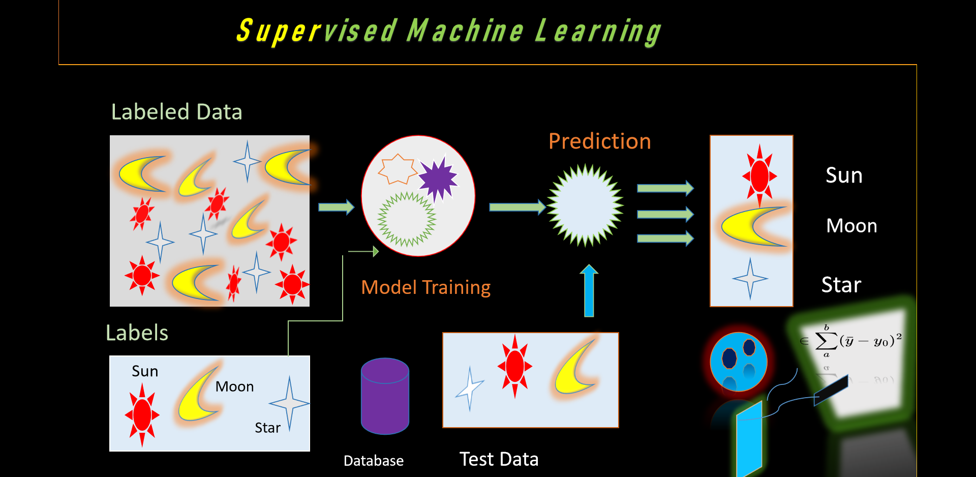Fig. Supervised Machine Learning

Let's study the Python codes in supervised ways .....

So, we are working in Python code along with pandas, seaborn, numpy etc. libraries to determine prediction on the basis of labeled data with supervised learning, we'll visualize the data and perform testing between various algorithms in the search of achieving higher accuracy.
Now let's discuss little bit about Supervised learning, it is a genre of machine learning and artificial intelligence that uses labeled datasets to train algorithms to predict outcomes and recognize patterns. Unlike unsupervised learning, supervised learning algorithms are given labeled training to learn the relationship between the input and the outputs.

So the question arises here, what is Supervised Machine Learning?... As per knowledge, supervised machine learning is a technique of machine learning in which it works on labeled data as we are seeing above figure that we have collection of labeled thing and we have to provide one input and find out the output from the given set right.
Atlast our aim is to construct a model which enable to learn from collected data and determine the predictions on the basis of prior data or unseen data right. If we talk about labeled data, then it comprise of input attribute said to be independent variables or predictors and the correlate with output docket said to be dependent variables or targets respectively. What is Supervised machine learning used for?...Basically our model's aim is to encapsulate patterns and correlation amidst the input attributes and the output docket, permits it to hypothesis and construct meticulously predicted features beside the unseen data respectively.

Algorithms

Let's study some of the algorithms present in supervised machine learning .....

1. Linear Regression

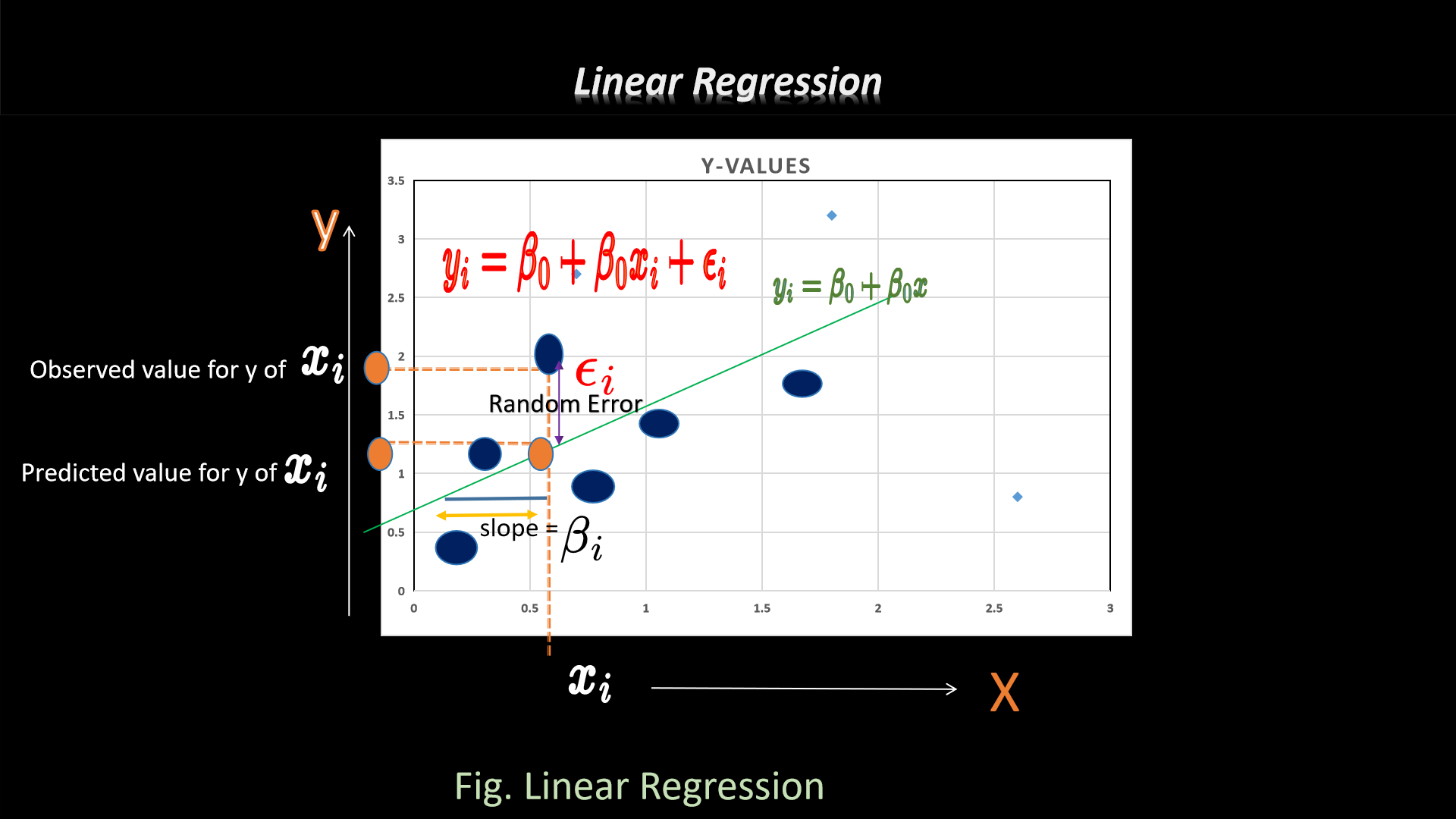
In general, linear regression is an analytical approach which is generally used to predict the consequences on the basis of prior collected information via interpreted mathematical formula to obtain desired output or else, we can say,prediction of unseen data searches from the collection of numerous data.
Basically it is a linear correlation between dependent and independent variables as we can see in fig. also.

Formula and its graphical representation::


y = β0 +β1x+ε

where, y_i = dependent variable
x_i = independent variable
B\beta = unknown parameters
e_i = error terms.


A scientifically tried-n-true prediction forecasting -

Generally, trafficking and trading kingpin can construct finer verdict via utilizing linear regression techniques. As per knowledge,ay firm poised stack of information, with the aid of linear regression utilizes such features for the finer maneuvering toward a desired result, in lieu expecting ahead of times and clairvoyance. Although folks, you grab bulk of raw info and recast to alter pragmatic particulars respectively.

Let's be familiar with some of the examples of Linear Regression ::
1. Evaluating trends and sales estimates
2. Analyze pricing elasticity
3.Assess risk in an insurance company
4. Sports analysis

2. support vector machines (SVM)

If we discuss about support vector machine (SVM), it is a kind of supervised learning algorithm, we can say, and utilized in machine learning to decode classification and regression stint. It's especially marvellous on puzzle out binary classification problems, that called for analyzing the facet concerning a database, articulate pairing cluster respectively. Generally employed for both classification or regression ultimatum. Although, SVM predominantly utilized in classification problems, like text classification.For example- handwriting recognitionintrusion detection, face detection, email classification, gene classification, and in web pages and also used in Cancer detection.

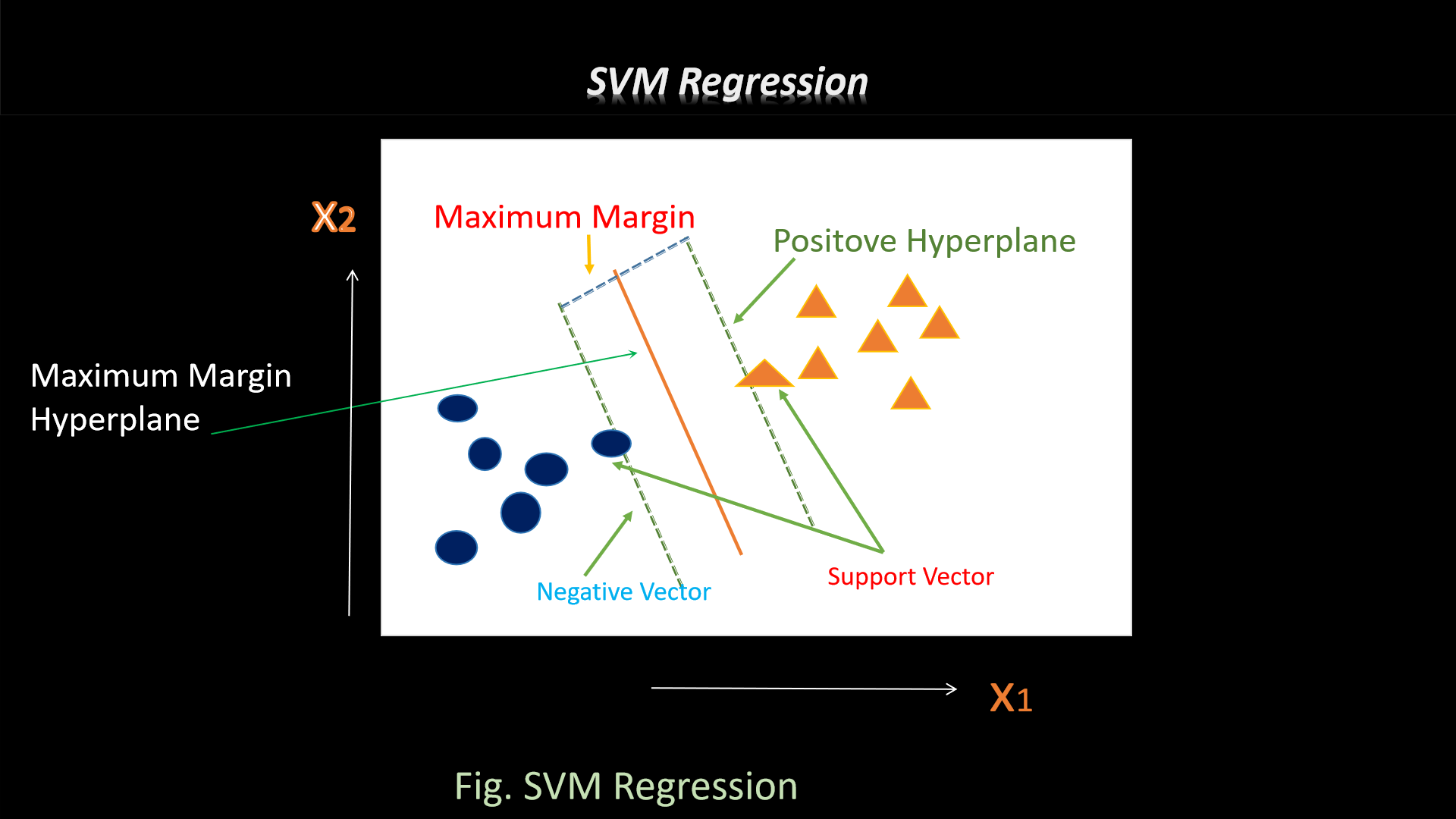
Formula for hyperplane and its graphical representation::


w^Tx+ b = 0


So, from the graphical representation, the equation of a hyperplane is w.x+b=0 where w said to be vector normal to hyperplane and b is an offset. When the value of w.x+b>0 it said to be a positive point or else negative point. After that we require (w,b) thats way the margin has a maximum distance.This function utilizedd to predict new values depends only on the support vectors.

One question arises that who pioneered SVM algorithm?.. So it's Vladimir N. Vapnik History. The SVM algorithm was discovered by Vladimir N. Vapnik and Alexey Ya. Chervonenkis in 1964

Let's be familiar with some advantages of SVM ::
1. Potent in high-dimensional specimen.
2. SVM's memory is logical as it utilizes a subset of training data during the decision function called support vectors.
3. Different kernel functions perhaps enumerated for the decision functions and its possible to enumerate custom kernels.

3. Decision Trees

Let's discuss little bit about decision tree. A decision tree algorithm is a machine learning algorithm which generally utilizes a decision tree to generate predictions on the basis of prior nodes. It comply with a tree-like structure called model of decisions and its feasible aftermaths. The algorithm functions near recursively rupturing the data into subsets on the basis of the most weighty attribute at each node of the tree respectively. 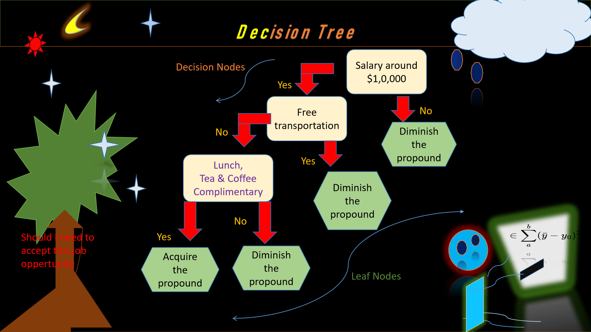Fig. Decision Trees Algorithms Graphical representations

Let's see some of the examples of a Decision Tree Algorithm ::

Forecasting ventures via prior weather info ::
Root node - Entire dataset
Attribute - (sunny, cloudy, rainy).
Subsets - Overcast, Rainy, and Sunny.
Iterative rupturing - Here, split up the sunny share especially as per humidity, like, Leaf Nodes - Persuit include “swimming,” “hiking,” and “staying inside.”

Somehow very helpful in choosing a sphere, tailing an education, considering a betterhalf, leading finances, and taking calculated menace are little bit leading decisions we generally confronting in esse. Thats why, momentous to take note, the decisions we are going to take in existence are inhabitually stubborn sincerely right.
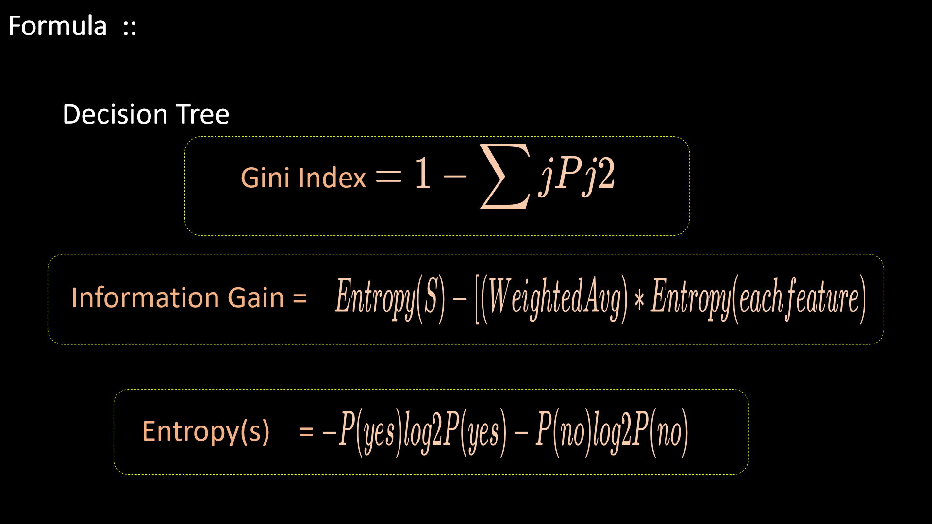
Where,
S= Total number of samples P(yes)= probability of yes P(no)= probability of no
Entropy: Entropy is a metric to measure the impurity in a given attribute. It specifies randomness in data. Entropy can be calculated as:

Advantages of Decision Tree

Now we are seeing how advantageous the decision tree as ::

1. It's easy to understand and interpret, producing ease to non-expertise.
2. Grasp both numerical and categorical data without requiring ample preprocessing.
3. Supplying insights towards facet urgency for decision-making.
4. Grasps null values and outliers without significant footprint.
5. Pertinent to both classification and regression tasks.

Disadvantages of Decision Tree

After that let's see disadvantages ::

1. The latent for overfitting.
2. Reactiveness to little changes in data.
3. Little stereotype, when training data is unillustrative.
4. The latent bias under the nose of divergence data.

4. K-nearest neighbor

Let's discuss about KNN said to be K-nearest neighbor (KNN) is a supervised machine learning algorithm. Generally KNN is uutilized to classify data points whilst it can accomplish regression too. The K-Nearest Neighbors Algorithm classify new data points to a discrete category rooted in its resemblance including further data points in such category. So the KNN algorithms seize the due to pick any useable configuration from the training data to portray the input data to the target data. Generally belongs to the category of nonparametric algorithms as doesn’t initiate any distinct premise regarding the mapping function.


dist(x,z)=(d∑r=1|xr−zr|p)1/p

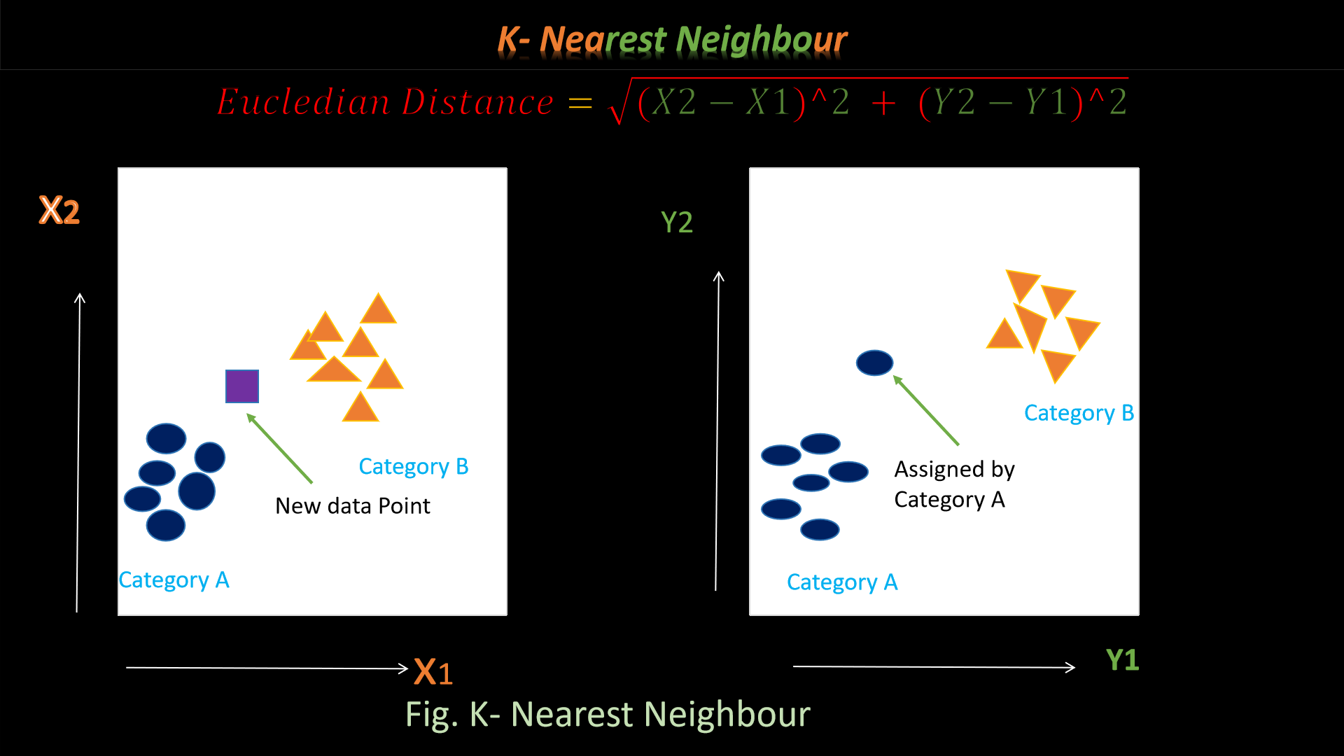
Working principle of KNN

1.Let's decide the number k in KNN.
2.After that, need to find out the parallelism based on Euclidean distance. K = formula
3.Then weigh the Euclidean distance of suspect point to K nearest neighbors
4.Finally, assign the class label to the suspect point

Underfitting and overfitting in KNN When the value is very small like K or K=2, the decision surface which separates different classes will not be smooth. The decision surface tries to make predictions with high accuracy in this case and it will lead to overfitting. On the other hand, when the value of is too high like , the decision surface itself vanishes and it results in a situation of classifying every query point as the majority class. This overly simplified assumption causes high bias and underfitting. Bias-variance trade-off has to be done with hyperparameter tuning of values in order to get a smooth decision surface. Smooth decision surfaces can guarantee an optimal model which neither overfit nor underfit. Such a decision surface will be less prone to noise.

Advantages of KNN

1. The potency of KNN grow accordingly with the huge training data and so it supports sufficient data representation.
2. KNN utilized for both classification and regression.
3. KNN is non parametric thatswhy speculation not linked with the basic input. Accordingly, nonlinear data also work well with it.
4. KNN Implementation is tranquil.

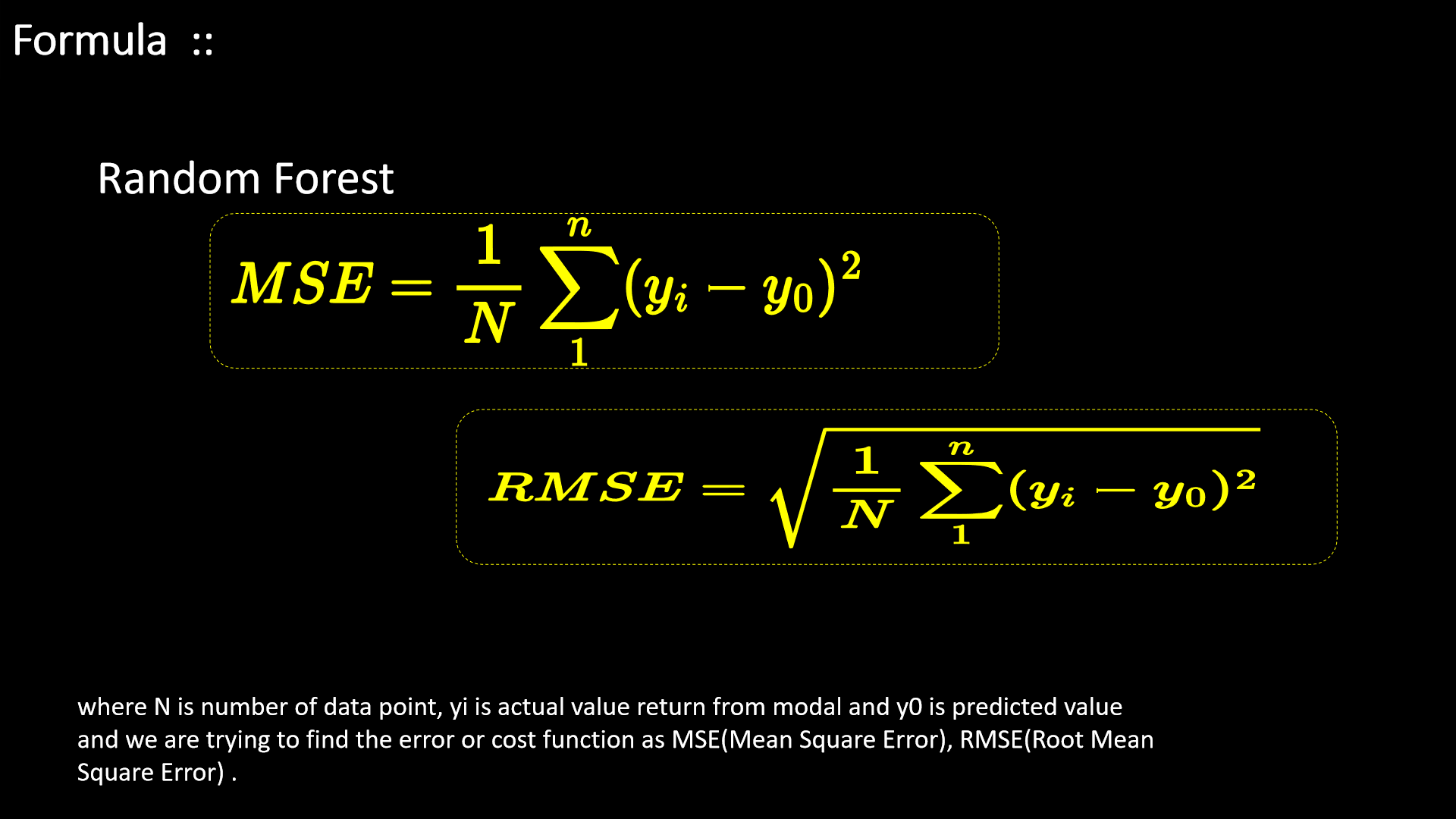
5. Random Forest

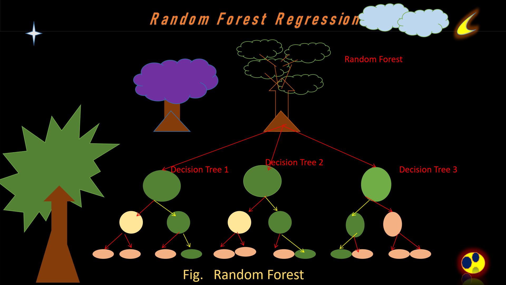
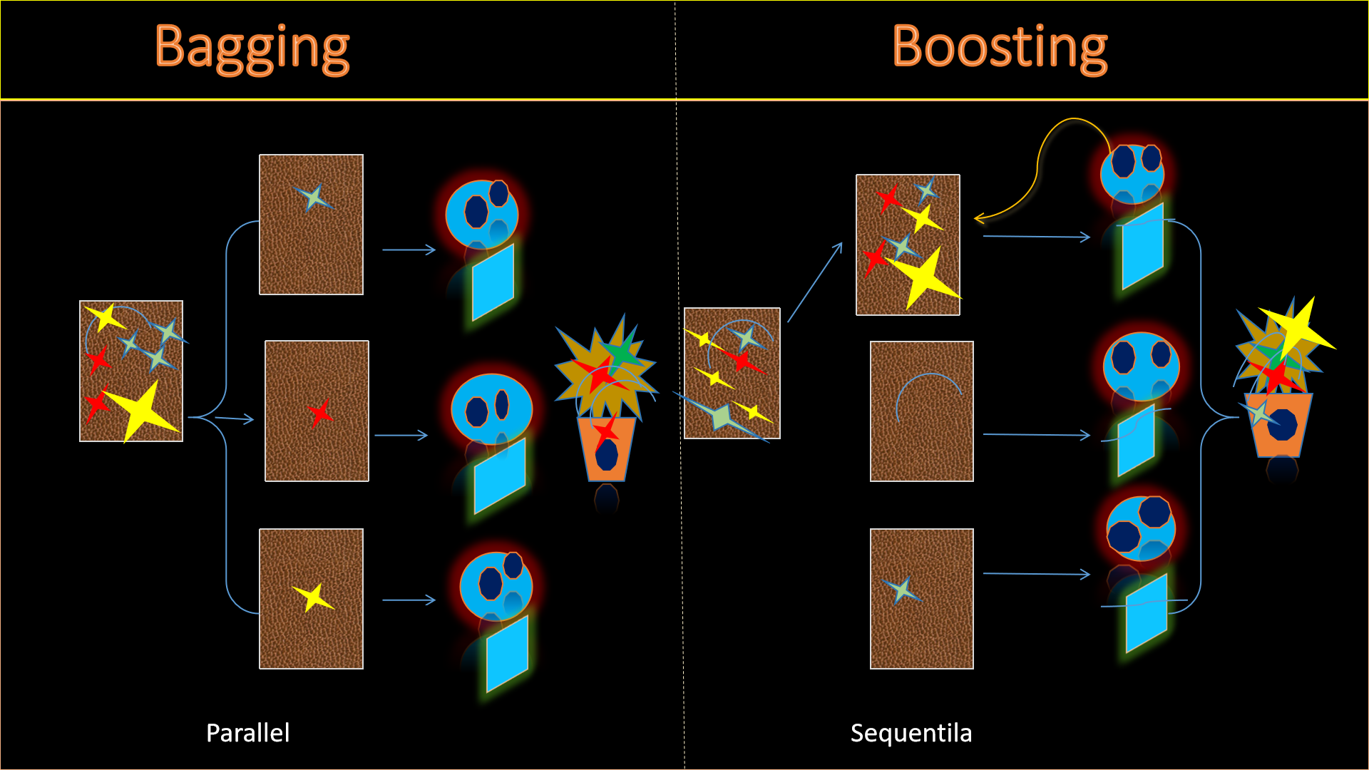
Let's discuss about Random Forest, a Random Forest Algorithm is a supervised machine learning algo which is vastly admired and is utilized for Classification and Regression problems. As per knowledge, a forest encompass innumerable trees, and the increased trees increases designed to occur robustness. Bagging :: While we generating a dissimilar training subset from sample training data with substitution is said to be Bagging. The closing output is organize according to mass voting. Another name of bagging is bootstrap aggregation, which ensemble learning method generally utilized to diminish variance enclosed by noisy dataset. Boosting :: On the other hand, mingling weak learners into strong learners by generating sequential models for instance the closing model having highest accuracy is said to be Boosting.
Random forests uses its default value . At the top of each pair is the probability that one of the relevant variables is chosen at any split. The results are based on 50 simulations for each pair, with a training sample of 300, and a test sample of 500

Let's be familiar with some of the examples of random forest :

1. Finance
2. E-commerce sector
3. Medical-Care

6. Naive-Bayes Classifier

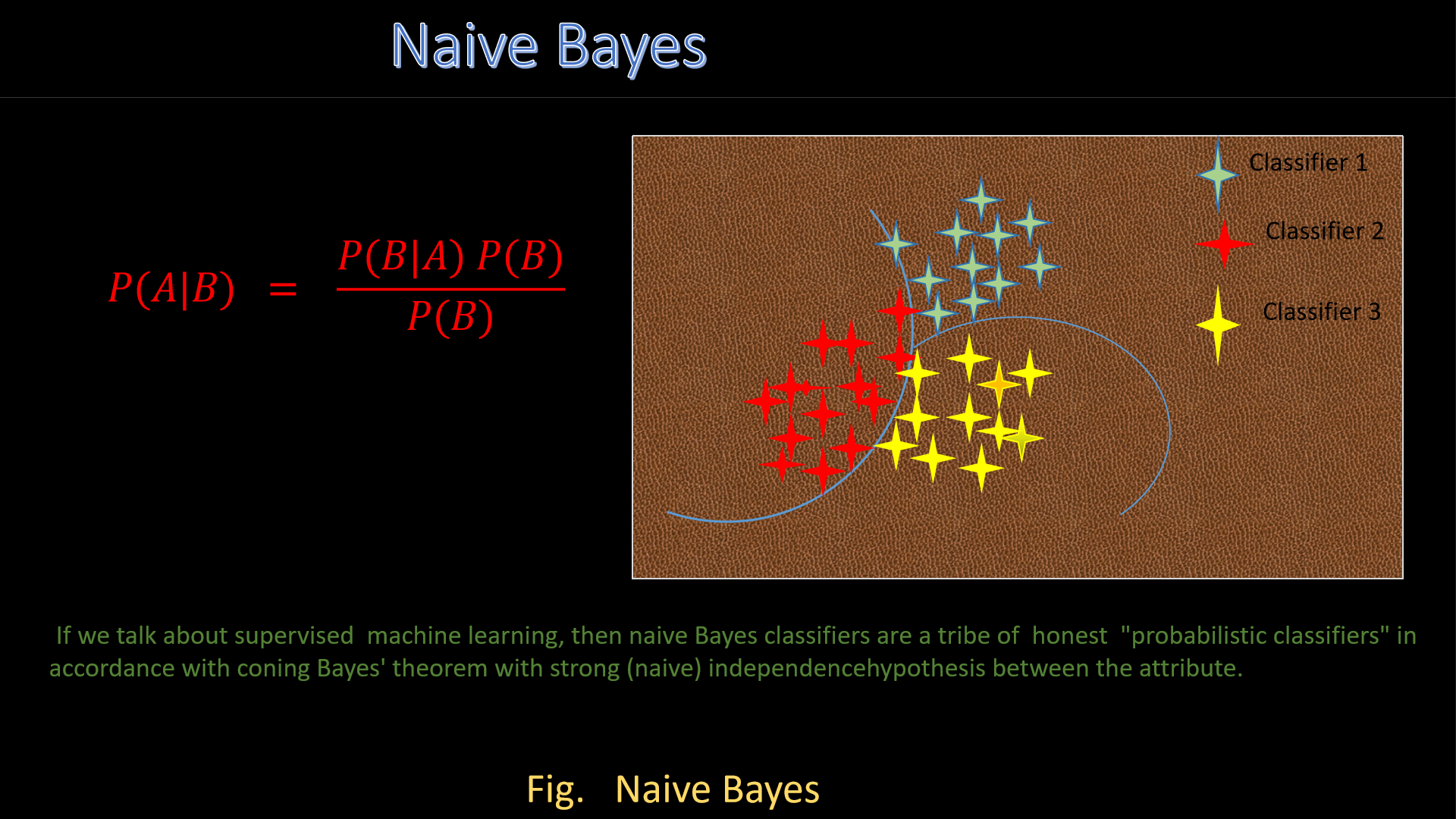
Now, let's see Naive Bayes, it's an algorithm which generally utilized Bayes' theorem to classify objects. Naive Bayes classifiers suppose strong, or naive, independence between feature of data points.

Let's be familiar with some of the examples of Naive-Bayes Classifier ::

1. Spam Filterig
2. Disease prediction
3. Document classificatio
4. Sentiment analysis
5. Mental state predictions

Advantages of Naive-Bayes

1. Less complex parameters are easier to estimate. As a result, it’s one of the first algorithms learned within data science and machine learning courses.
2. Scales well: Compared to logistic regression, Naïve Bayes is considered a fast and efficient classifier that is fairly accurate when the conditional independence assumption holds. It also has low storage requirements.
3. Can handle high-dimensional data: Use cases, such document classification, can have a high number of dimensions, which can be difficult for other classifiers to manage.

Disadvantages

1. Zero frequency occurs when a categorical variable does not exist within the training set.
2. While the conditional independence assumption overall performs well, the assumption does not always hold, leading to incorrect classifications.

7. Logistic Regression

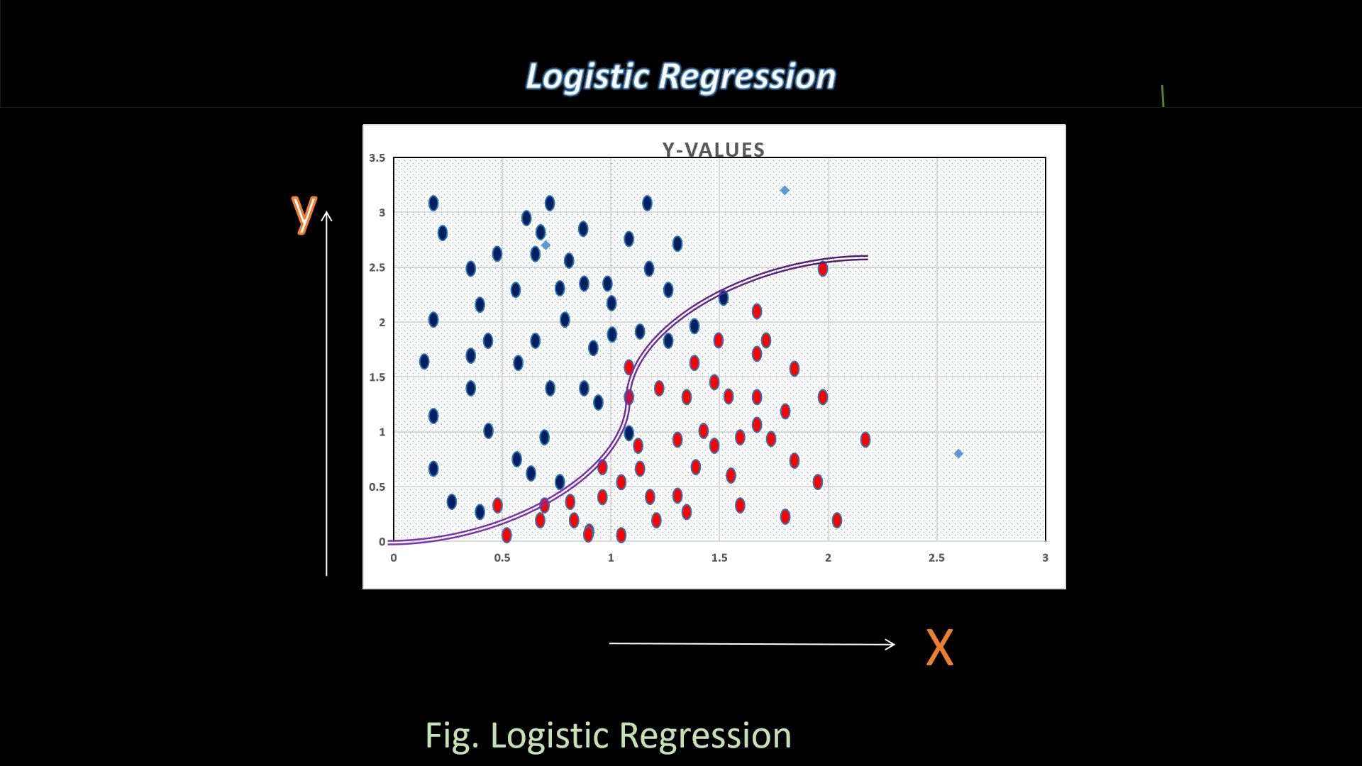
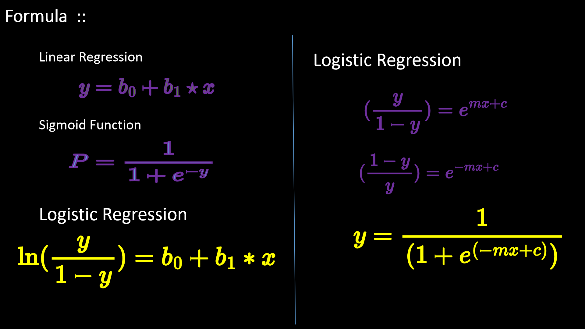
Let's understand Logistic regression, in accordance it is a supervised machine learning algorithm which attains binary classification tasks via forecasting the probability of an outcome, event, or observation. The model delivers a binary or dichotomous outcome limited to two possible outcomes: yes/no, 0/1, or true/false.

What is the uses?
Gaussian Distribution: Logistic regression is a linear algorithm (with a non-linear transform on output). It does assume a linear relationship between the input variables with the output. Data transforms of your input variables that better expose this linear relationship can result in a more accurate model.
Let's be familiar with some of the examples of Logistic Regression :

1. Fraud detection
2. Disease prediction
3. Churn prediction
4. Access credit risk
5. Banking sector profits rises rapidly

Let's implement the Python codes in supervised ways .....

# firstly we need to import required libraries

import pandas as pd
import numpy as np
import seaborn as sns
import matplotlib.pyplot as plt

Import csv file from our system for analysis

data = pd.read_csv('/content/drive/MyDrive/Housing.csv')

data

avb

result ::

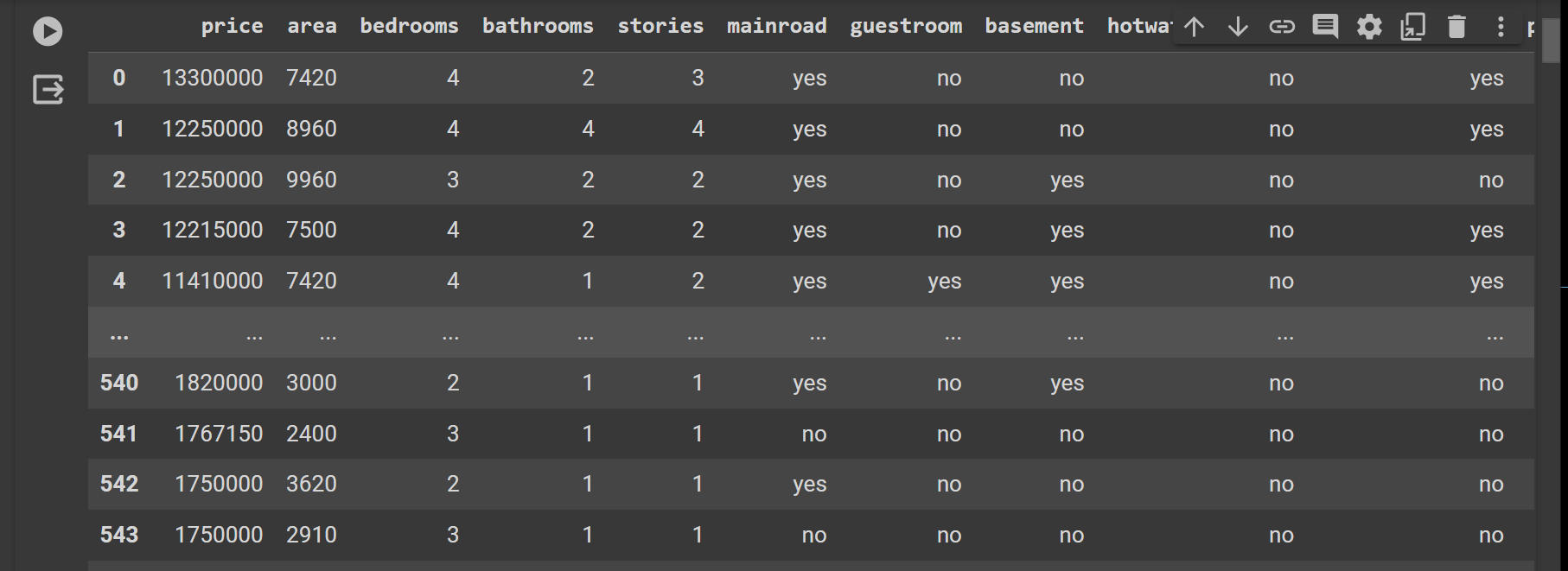
#now let's check the shape of our data

data.shape

result ::
(545, 13)

#now let's check the required information we needed during analysis

data.info()

result ::

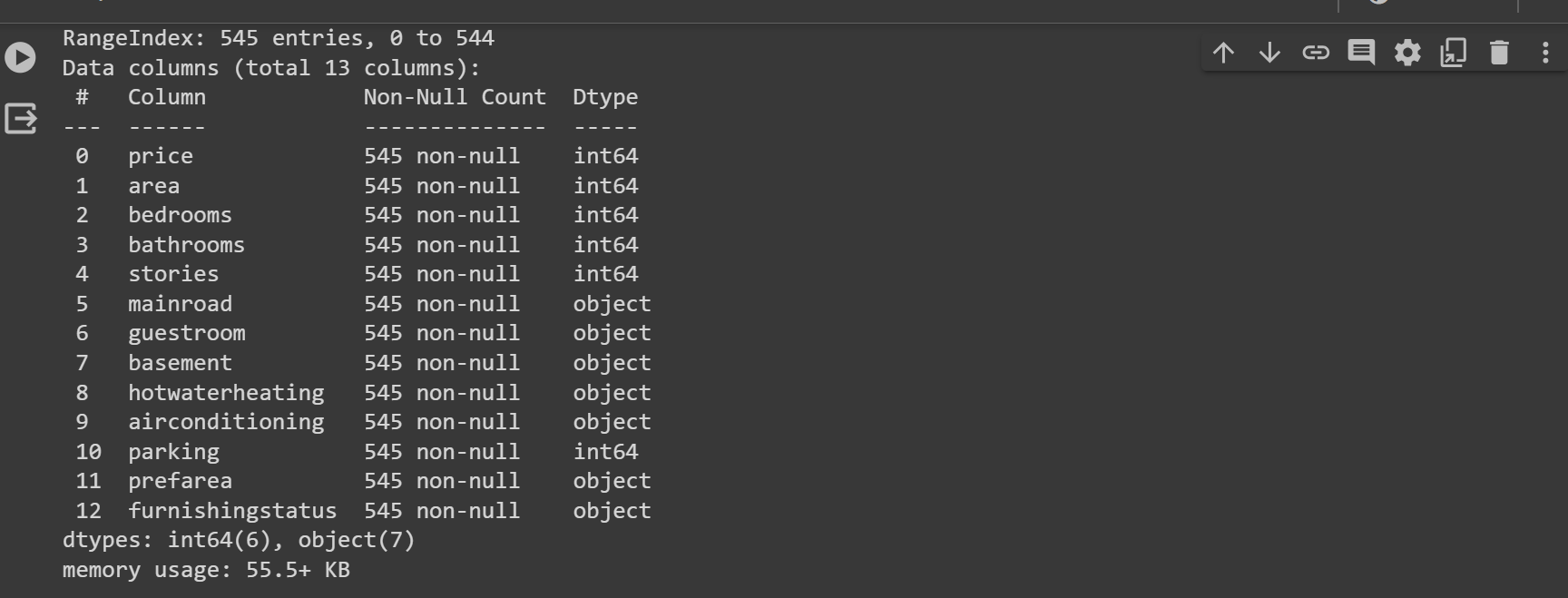
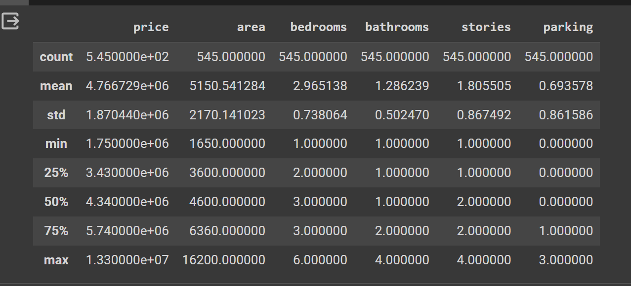
checking out detailed description of required data

data.describe()

result ::

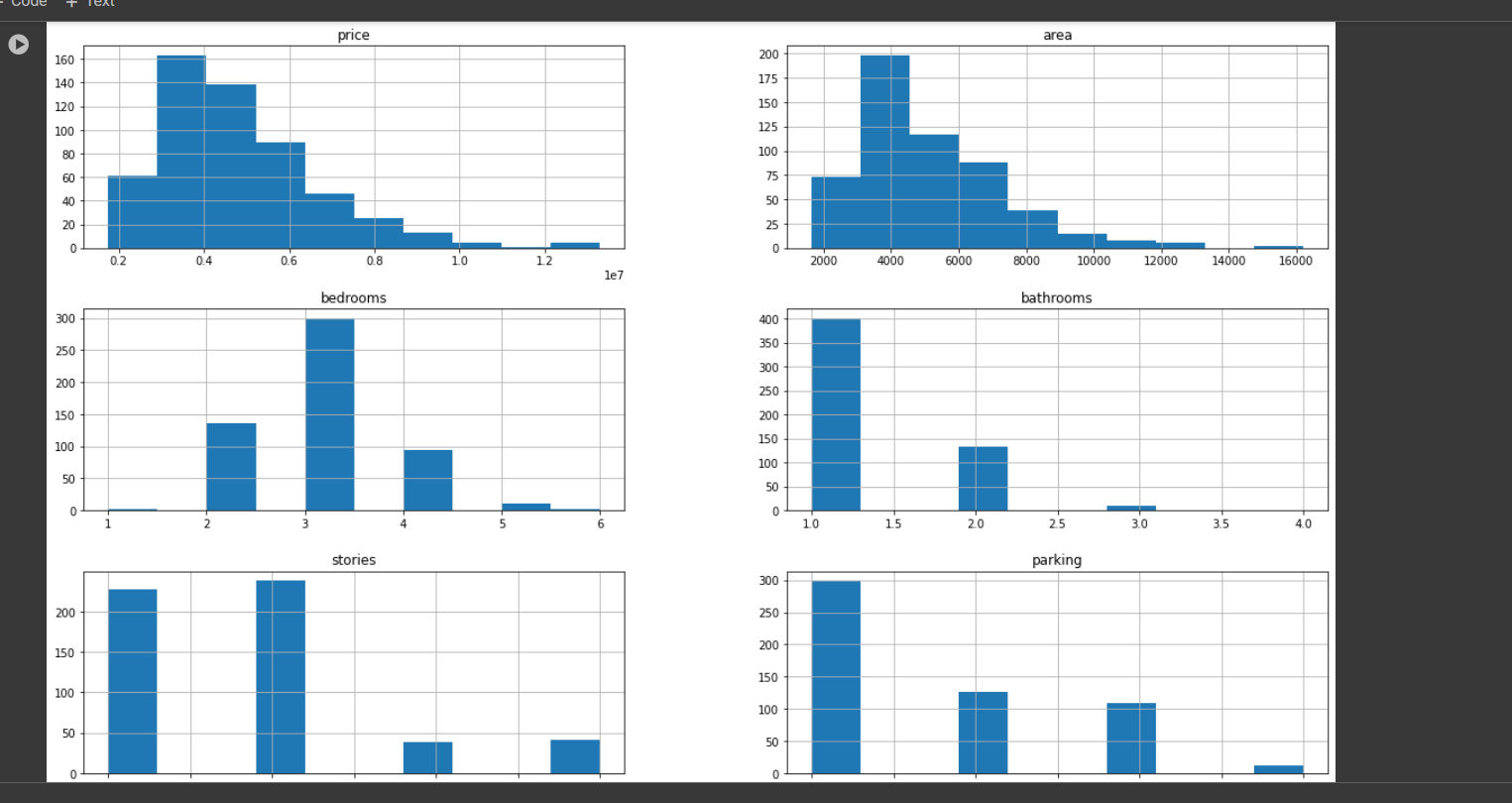
# now let's visualize the data via plotting, through graph we analyze in a better way

data.hist(figsize=(20,12)) plt.show()

result ::

# now let's checkout the null values so that we can replace with any otherwise it will give incorrect prediction

data.isnull()

result ::
​

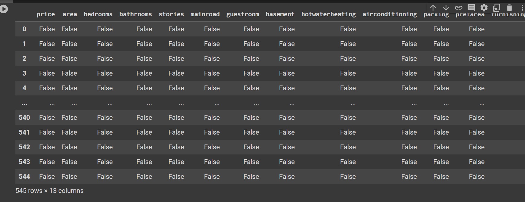
#now let's checkout the all null values prediction

data.isnull().sum()

result ::
​

# now we can split the data into test and train

training_data = data.drop(['price'], axis=1)

training_data

result ::

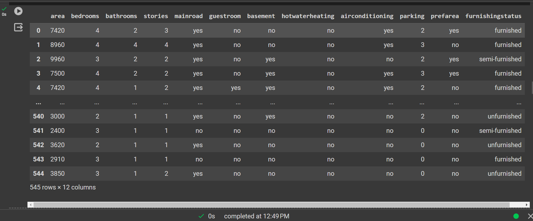
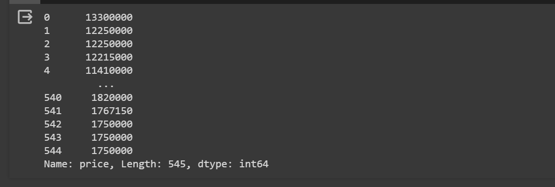
# now we can split the targrt data in which we have to do optimization

target_data = data['price']

target_data

result ::

from sklearn.model_selection import train_test_split

# now we can split it into the training and testing data for further testing optimization

train_data, test_data, y_train, y_test = train_test_split(training_data, target_data, test_size=0.2)

x_train, x_val, y, y_val = train_test_split(train_data, y_train, test_size=0.1)

DAta Processing

data.info()

result ::

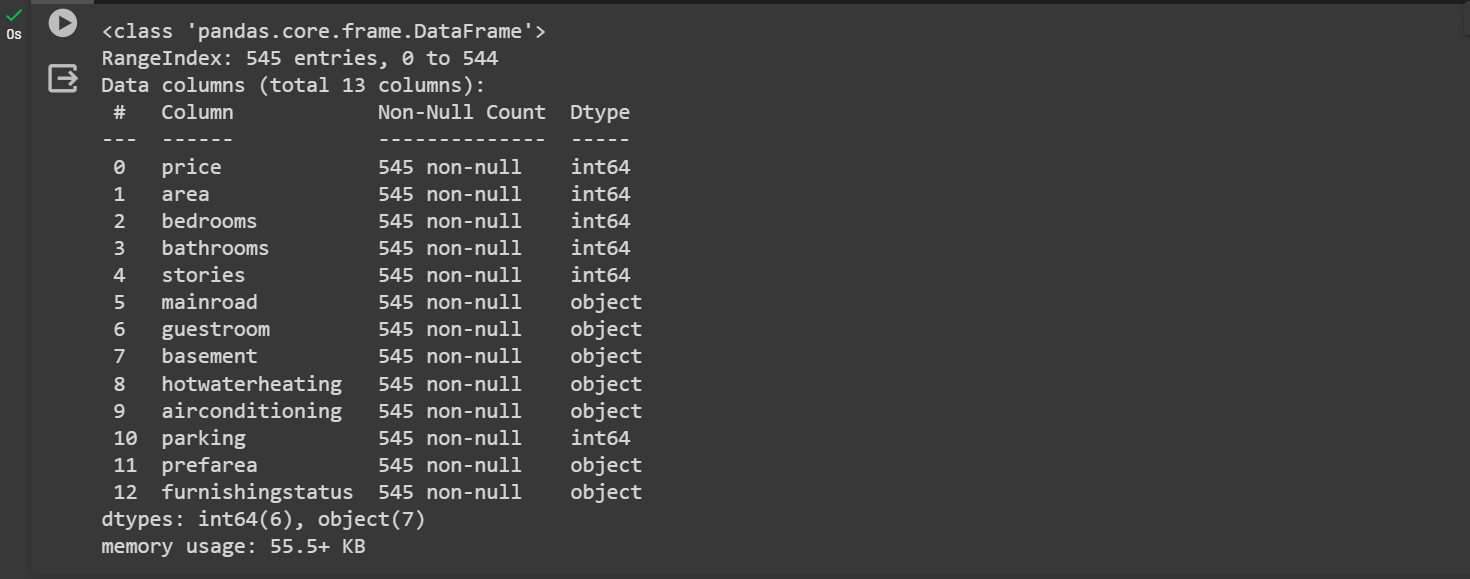
# now here we distinguish the numerical and categorical data separately
# OneHot Encoding performed here

num_attributes = ['area', 'bedrooms', 'bathrooms', 'stories', 'parking']

cat_attributes = ['mainroad', 'guestroom', 'basement', 'hotwaterheating', 'airconditioning', 'prefarea', 'furnishingstatus']

# now we import all other required libraries for implementing further supervised algorithm performance

from sklearn.preprocessing import StandardScaler, OneHotEncoder

from sklearn.pipeline import Pipeline

from sklearn.compose import ColumnTransformer

from sklearn.svm import SVR

from sklearn.linear_model import LinearRegression

from sklearn.tree import DecisionTreeRegressor

from sklearn.ensemble import RandomForestRegressor

from sklearn.metrics import mean_squared_error

num_pipeline = Pipeline([('std', StandardScaler())])

cat_pipeline = Pipeline([('onehotencoder', OneHotEncoder())])

full_pipeline = ColumnTransformer([('num', num_pipeline,num_attributes), ('cat', cat_pipeline, cat_attributes)])

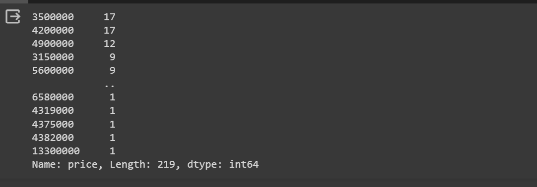
data['price'].value_counts()

result ::

data['price'].isnull().sum()

result ::
0

x_train = full_pipeline.fit_transform(x_train)

x_train.shape

result ::
(392, 20)

x_val = full_pipeline.transform(x_val)

test_data = full_pipeline.transform(test_data)

LInear Regression MOdel

lin_reg = LinearRegression()

lin_reg.fit(x_train, y)

result ::
LinearRegression
LinearRegression()

val_predictions = lin_reg.predict(x_val)

val_predictions

result ::
array ([ 7161701.38355163, 4245796.38410002, 4060017.98397319, 6992205.68674713, 6048031.03099421, 6537597.7074071 , 6943417.48381701, 4360500.53208898, 4500583.42804561, 4290132.96203464, 5715307.70241247, 4451108.83734066, 2947519.85144286, 3663781.87197194, 6074912.81245875, 4889085.05994701, 6618553.99455126, 5260882.40968955, 4139766.99635413, 6167454.82373424, 6434063.32717966, 3691697.37977568, 6659270.66905693, 4484284.33766644, 5123409.29319205, 3902141.50092292, 7475755.01711734, 4665420.67198095, 3582544.21087863, 2543505.44219759, 3065435.45200179, 4281985.71464318, 4487524.7073699 , 6849982.67921765, 6837073.33775704, 5552861.87496595, 2700334.77942049, 5871904.18372563, 5272117.30288319, 4135923.35948052, 2983756.75270146, 4479321.78900046, 6949138.7006256 , 8380901.37606378 ])

def return_rmse(targets, preds):
mse = mean_squared_error(targets, preds)

return np.sqrt(mse)

val_rmse = {}

test_rmse ={}

lin_reg_val_rmse = return_rmse(y_val, val_predictions)

val_rmse['Linear Regression'] = lin_reg_val_rmse

lin_reg_val_rmse

result ::
1045076.9408102289

lin_reg_test_preds =lin_reg.predict(test_data)

lin_reg_test_rmse = return_rmse(y_test, lin_reg_test_preds)

test_rmse['Linear Regression'] = lin_reg_test_rmse

lin_reg_test_rmse

result ::
889693.2600628015

SVM regression or Support Vector Regression (SVR) is a machine learning algorithm used for regression analysis. It is different from traditional linear regression methods as it finds a hyperplane that best fits the data points in a continuous space, instead of fitting a line to the data points.
SVR with a linear kernel is more robust than Linear Regression as it doesn't make as many assumptions.


SVR

svr = SVR()

svr.fit(x_train, y)

result ::
SVR
SVR()

svr_val_preds = svr.predict(x_val)
svr_val_rmse = return_rmse(svr_val_preds, y_val)
val_rmse['SVR'] = svr_val_rmse
svr_val_rmse

result ::
2008427.3480822272

svr_test_preds = svr.predict(test_data)
svr_test_rmse = return_rmse(svr_test_preds, y_test)
test_rmse['SVR'] = svr_test_rmse
svr_test_rmse

result ::
1753860.5503273602

DecisionTree

tree_reg = DecisionTreeRegressor()
tree_reg.fit(x_train, y)

result ::
DecisionTreeRegressor
DecisionTreeRegressor()

tree_val_preds = tree_reg.predict(x_val)
tree_val_rmse = return_rmse(tree_val_preds, y_val)
val_rmse['Decision Tree'] = tree_val_rmse
tree_val_rmse

result ::
1726335.9122193402

tree_test_preds = tree_reg.predict(test_data)
tree_test_rmse = return_rmse(tree_test_preds, y_test)
test_rmse['Decision Tree'] = tree_test_rmse
tree_test_rmse

result ::
1642502.4058323742

#Random Forest

forest_reg = RandomForestRegressor()
forest_reg.fit(x_train, y)

result ::
RandomForestRegressor
RandomForestRegressor()

forest_val_preds = forest_reg.predict(x_val)
forest_val_rmse = return_rmse(forest_val_preds, y_val)
val_rmse['Random Forest'] = forest_val_rmse
forest_val_rmse

result ::
1051281.1430706223

forest_test_preds = forest_reg.predict(test_data) forest_test_rmse = return_rmse(forest_test_preds, y_test) test_rmse['Random Forest'] = forest_test_rmse forest_test_rmse

result ::
968434.6715352592

#Comparision between Models

val_rmse

result ::
{'Linear Regression': 1045076.9408102289,
'SVR': 2008427.3480822272,
'Decision Tree': 1726335.9122193402,
'Random Forest': 1051281.1430706223}

test_rmse

result ::
{'Linear Regression': 889693.2600628015,
'SVR': 1753860.5503273602,
'Decision Tree': 1642502.4058323742,
'Random Forest': 968434.6715352592}

sorted(val_rmse.items(), key=lambda x:x[1])

result ::
[('Linear Regression', 1045076.9408102289),
('Random Forest', 1051281.1430706223),
('Decision Tree', 1726335.9122193402),
('SVR', 2008427.3480822272)]

sorted(test_rmse.items(), key=lambda x:x[1])

result ::
[('Linear Regression', 889693.2600628015),
('Random Forest', 968434.6715352592),
('Decision Tree', 1642502.4058323742),
('SVR', 1753860.5503273602)]

Applications of Supervised Machine Learning

Spam Email Detection

So basically supervised learning can be utilized to analyze emails as spam may admissible. Close to training our model approaching a labeled dataset regarding spam and non-spam emails, so this accurately envision in case an arriving email concluded to be spam, via utilizing this, allocate displeasing e-mail messages.

Wellness program set-up:

Here Python simulations generally used a blueproint hospital workflows, patient flows, andSpam Email Detection stock allocation.By simulating various tasks, healthcare contributer perhaps recognize tailback, enhance stock utilization, and maximize patient follow-up. Python simulation visualization tools like Matplotlib and Plotly permit distinct portrayal of data and ease decision-making startegy.

Transit and Plannings:

So if we talk about business aesthetics, in transportation, we simulating logistics performance, traffic flow or supply chain networks assist maximize transportation systems.Generally python simulations empower orgaizations to recognize highest routes, evaluate the footprint of framework transpose, and improve stock allocation. Real-time visualization of simulations using libraries like Bokeh or Plotly permits collaborator construct data-driven decisions on the dot.

Some other applications and advantages are written below ::

Bioinformatics

Cheminformatics

Quantitative structure–activity relationship

Database marketing

Handwriting recognition

Information retrieval

Learning to rank

Information extraction

Object recognition in computer vision

Optical character recognition

Pattern recognition

Speech recognition

Supervised learning is a special case of downward causation in biological systems

Landform classification using satellite imagery

Spend classification in procurement processes

Limitations of Supervised Learning

Let's see some of the limititions or disadvantages of supervised learning ::

1. Unable to grasp all complex tasks
2. Computation time is gigantic
3. Shortfall of training data
4. Inferior standard of data
5. Data overfitting
6. Data underfitting
7. Lower plasticity and slight performance in non-stop learning scenarios.

References

1. C.E. Brodely and M.A. Friedl (1999). Identifying and Eliminating Mislabeled Training Instances, Journal of Artificial Intelligence Research 11, 131-167. (http://jair.org/media/606/live-606-1803-jair.pdf)

2. Wikipedia

3. IBM social sites